Machine Learning Basics(1): Linear Regression

As a beginner in machine learning, I plan to sketch out my learning process. And it will be my first post in this series.

1. Definition

We have an input vector $X^T=(X_1, X_2, \dots, X_p)$ and want to predict a real-valued output $Y$. The linear regression model has the form

$f(X)=\beta_0 + \sum_{j=1}^pX_j\beta_j.\quad(1.1)$

Here the $\beta_j$’s are unknown parameters or coefficients.

2. Least Squares

Typically we have a set of training data $(x_1,y_1)\dots(x_N,y_N)$ from which to estimate the parameters $\beta$. The most popular estimation method is least squares, in which we pick the coefficients $\beta=( \beta_0, \beta_1, \dots, \beta_p)^T$ to minimize the residual sum of squares (RSS)

$RSS(\beta)=\sum_{i=1}^N(y_i-f(x_i))^2.\quad(2.1)$

How do we minimize $(2.1)$? This is an important question with a beautiful answer. The best $\beta$ can be found by geometry or algebra or calculus. Let’s explain the three approaches one by one.

Calculus Interpretation

Denote by $\mathbf{X}$ the $N\times (p+1)$ matrix with each row an input vector (with a 1 in the first position). We can rewrite $(2.1)$ in the matrix form as

$RSS(\beta)=(\mathbf{y}-\mathbf{X}\beta)^T(\mathbf{y}-\mathbf{X}\beta).\quad(2.2)$

This is a quadratic function in the $p+1$ parameters. Differentating with respect to $\beta$ we obtain

$\frac{\partial RSS}{\partial\beta}=-2\mathbf{X}^T(\mathbf{y}-\mathbf{X}\beta).\quad(2.3)$

In order to get the minimum RSS, we set the first derivative to zero

$\mathbf{X}^T(\mathbf{y}-\mathbf{X}\beta)=0\quad(2.4)$

to obtain the unique solution

$\hat\beta = (\mathbf{X}^T\mathbf{X})^{-1}\mathbf{X}^T\mathbf{y}.\quad(2.5)$

The fitted values are

$\mathbf{\hat y}=\mathbf{X}\hat\beta=\mathbf{X}(\mathbf{X}^T\mathbf{X})^{-1}\mathbf{X}^T\mathbf{y}.\quad(2.6)$

One thing which should be noticed is that it’s wrong to split $(\mathbf{X}^T\mathbf{X})^{-1}$ into $\mathbf{X}^{-1}$ times $\mathbf{X}$ and cancel the terms before $\mathbf{y}$ in $(2.6)$. The matrix $\mathbf{X}$ is rectangualr and has no inverse matrix. And if $\mathbf{X}$ is square and invertible, $\mathbf{\hat y}$ is exactly $\mathbf{y}$ just as $(2.6)$ shows.

Someone may be confused by how to get $(2.3)$ by $(2.2)$ just as I once experienced. Actually, the easiest way to figure it out is to differentiate with respect to each $\beta_j$ respectively

$\begin{split}\frac{\partial RSS}{\partial\beta_j}&=\frac{\partial}{\partial\beta_j}\sum_{i=1}^N\left(y_i-\sum_{j=0}^px_{ij}\beta_j\right)^2 \\ &=-2\sum_{i=1}^Nx_{ij}\left(y_i-\sum_{j=0}^px_{ij}\beta_j\right). \\ \end{split}$

Then, we put all the derivatives together and rewrite it in matrix form to get $(2.3)$.

Geometry Interpretation

Alt text

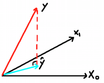
The picture above shows a direct gemotrical representation of the least squares estimate with two predictors. It’s convenient to extend this to the case with more predictors. We denote the column vectors of $X$ by $\mathbf{x}_0,\mathbf{x}_1,\dots,\mathbf{x}_p$ with $\mathbf{x}_0 \equiv 1$. These vectors span a subspace of $\mathbb{R}^N$, also referred to as the column space of $\mathbf{X}$. We minimize $RSS(\beta)=\lVert\mathbf{y}-\mathbf{X}\beta\rVert^2$ by choosing $\hat \beta$ so that the residual vector $\mathbf{y}-\mathbf{\hat y}$ is orthogonal to this subspace. This orthogonality is expressed in $(2.4)$, and the resulting estimate $\mathbf{\hat y}$ is hence the orthogonal projection of $\mathbf y$ onto this subspace.

Algebra Interpretation

In the world of linear algebra, we will also view our problem from a perspective of algebra. Now we reformulate the problem as to solve the linear equations system $\mathbf{X}\beta=\mathbf{y}$. If you are somewhat familar with linear algebra, you can try to use elimination to solve it. Unfortunately, it has no solution typically due to there are more equations than unknowns ($n$ is larger than $p$).

Instead, we hope that the length of error $\mathbf{e}=\mathbf{y}-\mathbf{X}\hat\beta$ is as small as possible. And the corresponding $\hat\beta$ is a least squares solution.

When $\mathbf{X}\beta=\mathbf{y}$ has no solution, we can multiply by $\mathbf{X}^T$ and solve $\mathbf{X}^T\mathbf{X}\beta=\mathbf{X}^T\mathbf{y}$. And it yields the solution from calculus exactly. In the language of algebra, we can split the $\mathbf{y}$ into two parts as $\mathbf{p}+\mathbf{e}$. The part in the column space is $\mathbf{p}$. The perpendicular part in the nullspace of $\mathbf{X}^T$ is $\mathbf{e}$. There is an equation we cannot solve ($\mathbf{X}\beta=\mathbf{y}$). There is an equation $\mathbf{X}\hat\beta=\mathbf{p}$ we do solve. And the solution to $\mathbf{X}\hat\beta=\mathbf{p}$ leaves the least possible error. How do we choose $\mathbf{p}$ in the column space? Just as the geometry part tells us, the projection of $\mathbf{y}$ onto the column space!

Ok, now the three interpretations come together and form a complete picture for the least squares.

Wait a minute, there is still one more question. It might happen that that the columns of $\mathbf{X}$ are not linearly independent, so that $\mathbf{X}$ is not of full rank. Then $\mathbf{X}^T\mathbf{X}$ is singular and the least squares coefficients $\hat\beta$ are not uniquely defined. However, the fitted values $\mathbf{\hat y}=\mathbf{X}\hat\beta$ are still the projection of $\mathbf{y}$ onto the column space of $\mathbf{X}$; there is just more than one way to express that projections in terms of the column vectors of $\mathbf{X}$.

3. Implementations

The implementations is extremely easy in a language like R, even without specific packages. The core code is shown below:

library(MASS)
betaHat <- ginv(t(X) %*% X) %*% t(X) %*% y
yhat <- X %*% betaHat

You can also use packages like lm in R. It provides not only $\hat\beta$ but also a lot sophisticated coefficients.

4. Taste on Statistics

To be continued

Billy Ian's Short Leisure-time Wander

into learning, investment, intelligence and beyond