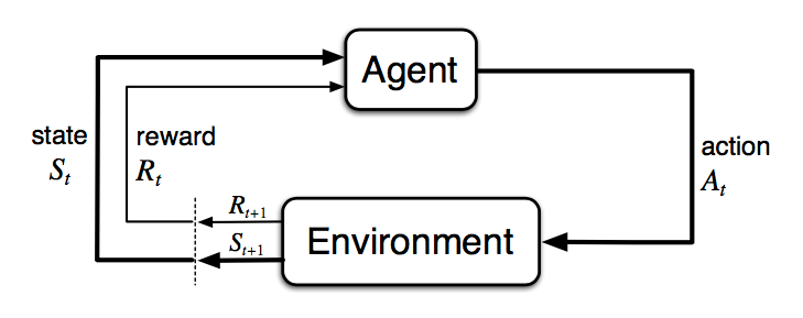
The Agent-Environment Interface

• The agent and environment interact at each of a sequence of discrete time steps, $t=0,1,2,3,\dots$
• At each time step $t$, the agent receives some representation of the environment’s state, $S_t\in\mathcal{S}$, where $\mathcal{S}$ is the set of possible states.
• On that basis, the agent selects an action, $A_t \in \mathcal{A}(S_t)$, where $\mathcal{A}(S_t)$ is the set of actions available in state $S_t$.
• One time step later, in part as a consequence of its action, the agent receives a numerical reward, $R_{t+1} \in \mathcal{R} \subset \mathbb{R}$, and finds itself in a new state, $S_{t+1}$.

At each time step, the agent implements a mapping from states to probabilities of selecting each possible action. This mapping is called the agent’s policy and is denoted $\pi_t$, where $\pi_t(a \vert s)$ is the probability that $A_t=a$ if $S_t=s$. Reinforcement learning methods specify how the agent changes its policy as a result of its experience. The agent’s goal, roughly speaking, is to maximize the total amount of reward it receives over the long run.

The general rule we follow is that anything that cannot be changed arbitrarily by the agent is considered to be outside of it and thus part of its environment.

Rewards and Returns

At each time step, the reward is a simple number, $R_t \in \mathbb{R}$. Informally, the agent’s goal is to maximize the total amount of reward it receives. If the sequence of rewards received after time step $t$ is denoted $R_{t+1}, R_{t+2}, R_{t+3}, \dots$, we seek to maximize the expected return, where the return $G_t$ is defined as some specific function of the reward sequence.

Here we define the return as:

$$G_t = \sum_{k=0}^{T-t-1}\gamma^kR_{t+k+1}$$

where $T$ can be $\infty$ and $0<\gamma\le1$ is the discounting rate.

Markov Decision Processes

A reinforment learning task that satisfies the Markov preperty is called a Markov decision process, or MDP. If the state and action spaces are finite, then it is called a finite Markov decision process (finite MDP).

Given any state and action $s$ and $a$, the probability of each possible pair of next state and reward, $s’$, $r$, is denoted

$$p(s',r|s,a)=\Pr\{S_{t+1}=s',R_{t+1}=r|S_t=s,A_t=a\}.$$

These quantities completely specify the dynamics of a finite MDP.

Value Functions

The value of a state $s$ under a policy $\pi$, denoted $v_\pi(s)$, is the expected return when starting in $s$ and following $\pi$ thereafter. For MDPs, we can define $v_\pi(s)$ formally as

$$v_\pi(s)=\mathbb{E}_\pi[G_t|S_t=s]=\mathbb{E}_\pi\left[\sum_{k=0}^\infty\gamma^kR_{t+k+1}\middle|S_t=s\right],$$

where $\mathbb{E}[\centerdot]$ denotes the expected value of a random variable given that the agent follows policy $\pi$, and $t$ is any time step. We call the function $v_\pi$ the state-value function for policy $\pi$.

Similarly, we define the value of taking action $a$ in state $s$ under a policy $\pi$, denoted $q_\pi(s,a)$, as the expected return starting from $s$, taking the action $a$, and thereafter following policy $\pi$:

$$q_\pi(s,a)=\mathbb{E}_\pi[G_t|S_t=s,A_t=s]=\mathbb{E}_\pi\left[\sum_{k=0}^\infty\gamma^kR_{t+k+1}\middle|S_t=s,A_t=a\right].$$

We call $q_\pi$ the action-value function for policy $\pi$.

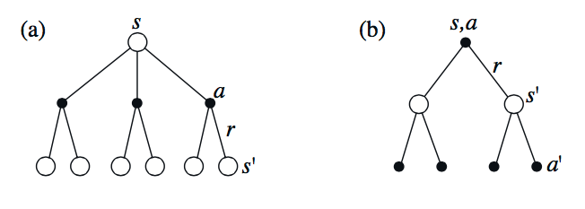
A fundamental property of value functions used throughout reinforcement learning and dynamic programming is that they satisfy particular recursive relationships. For any policy $\pi$ and any state $s$, the following consistency condition holds between the value of $s$ and the value of its possible successor states:

$$v_\pi(s)=\sum_a\pi(a|s)\sum_{s',r}p(s',r|s,a)[r+\gamma v_\pi(s')], \forall s \in \mathcal{S}.$$

This equation is the Bellman equation for $v_\pi$. Likewise, the Bellman equation for action values $q_\pi$ is as follows:

$$q_\pi(s,a)=\sum_{s',r}p(s',r|s,a)[r+\gamma\sum_{a'}\pi(a'|s')q(s',a')]$$

According to the Bellman equations, we can derive the relatioship between $v_\pi$ and $q_\pi$:

$$\begin{split} v_\pi(s)&=\mathbb{E}_\pi[q_\pi(S_{t}, a)|S_t=s]\\ &= \sum_a\pi(a|s)q_\pi(s,a) \end{split}$$ $$\begin{split} q_\pi(s, a)&=\mathbb{E}[R_{t+1}+\gamma v_\pi(S_{t+1})|S_t=s, A_t=a]\\ &=\sum_{s',r}p(s',r|s,a)[r+\gamma v_\pi(s')] \end{split}$$

Optimal Value Functions

A policy $\pi$ is defined to be better than or equal to a policy $\pi’$ if its expected return is greater than or equal to that of $\pi’$ for all states. In other words, $\pi\ge\pi’$ if and only if $v_\pi(s)\ge v_{\pi’}(s)$ for all $s\in\mathcal{S}$. There is always at least one policy that is better than or equal to all other policies. This is an optimal policy $\pi_*$.

The optimal state-value function, denoted $v_*$, are defined as

$$v_*(s) = \max_\pi v_\pi(s),$$

for all $s\in\mathcal{S}$.

The optimal action-value function, denoted $q_*$, are defined as

$$q_*(s,a)=\max_\pi q_\pi(s,a),$$

for all $s\in\mathcal{S}$ and $a\in\mathcal{A}(s)$.

The Bellman optimalality equation for $v_$ and $q_$ is

$$\begin{split} v_*(s)&=\max_a\mathbb{E}_\pi[R_{t+1}+\gamma v_*(S_{t+1})|S_t=s, A_t=a]\\ &= \max_{a\in\mathcal{A}(s)}\sum_{s',r}p(s',r|s,a)[r+\gamma v_*(s')] \end{split}$$ $$\begin{split} q_\pi(s, a)&=\mathbb{E}\left[R_{t+1}+\gamma q_*(S_{t+1},a')\middle|S_t=s, A_t=a\right]\\ &=\sum_{s',r}p(s',r|s,a)[r+\gamma \max_{a'}q_*(s',a')] \end{split}$$