Monte Carlo methods are ways of solving the reinforcement learning problem based on averaging sample returns. To ensure that well-defined returns are available, here we define Monte Carlo methods only for episodic tasks.

Monte Carlo Prediction

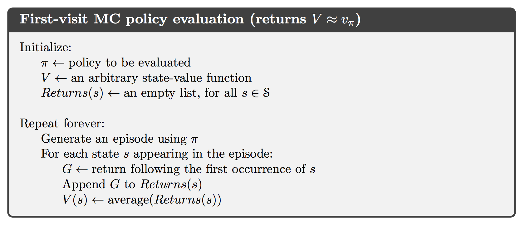
An obvious way to estimate the state-value function which is the expected return starting from that state from experience, is to average the returns observed after visits to that state. This idea underlies all Monte Carlo methods.

In particular, suppose we wish to estimate $v_\pi(s)$, the value of a state $s$ under policy $\pi$, given a set of episodes obtained by following $\pi$ and passing through $s$. Each occurrence of state $s$ in an episode is called a visit to $s$. The first-visit MC method estimates $v_\pi(s)$ as the average of the returns following from first visits to $s$, whereas every-visit MC method averages the returns following all visits to $s$.

An important fact about Monte Carlo method methods is that the estimates for each state are independent. The estimate for one state does not build upon the estimate of any other state, as is the case in DP.

Monte Carlo Estimation of Action Values

If a model is not available, then it is particularly useful to estimate action values rather than state values. The Monte Carlo methods for this this are essentially the same as just presented for state values, except now we talk about visits to a state–action pair rather than to a state. A state–action pair $s, a$ is said to be visited in an episode if ever the state $s$ is visited and action $a$ is taken in it.

The only complication is that many state–action pairs may never be visited. This is the general problem of maintaining exploration.

Monte Carlo Control

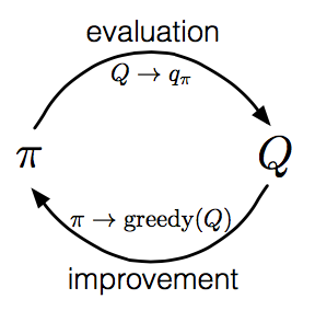
The overall idea of how Monte Carlo estimation can be used in control is to according to the idea of generalized policy iteration (GPI). In GPI one maintains both an approximate policy and an approximate value function. The value function is repeatedly altered to more closely approximate the value function for the current policy, and the policy is repeatedly improved with respect to the current value function.

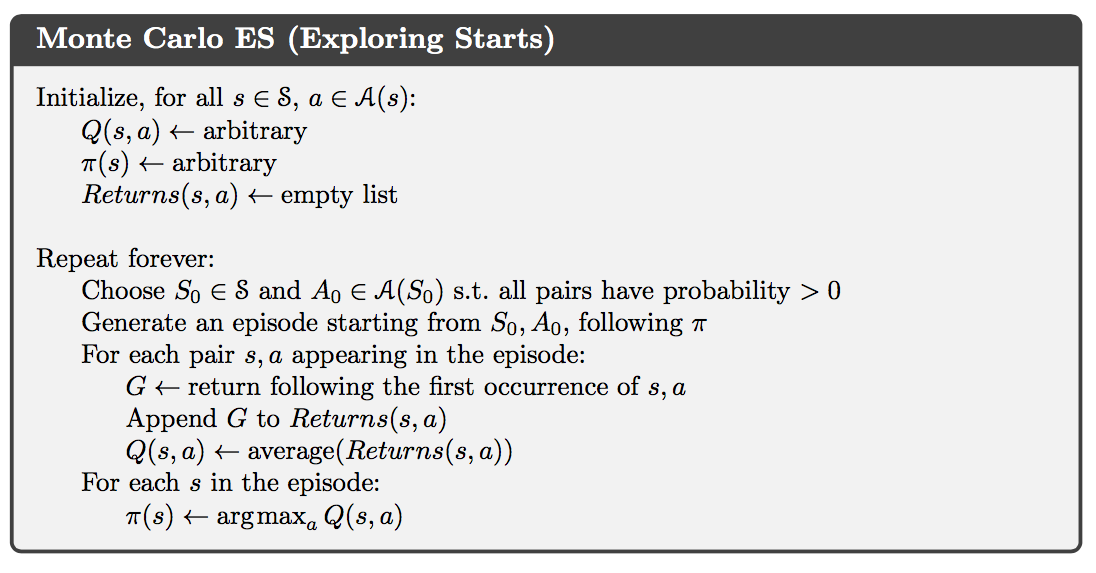
We made two unlikely assumptions in order to easily obtain guarantee of convergence for the Monte Carlo method. One was that the episodes have exploring starts, and the other was that policy evaluation could be done with an infinite number of episodes.

The assumption that policy evaluation operates on an infinite number of episodes are relatively easy to remove. One of the approaches it to forgo trying to complete policy evaluation before returning to policy improvement. For Monte Carlo policy evaluation it is natural to alternate between evaluation and improvement on an episode-by-episode basis.

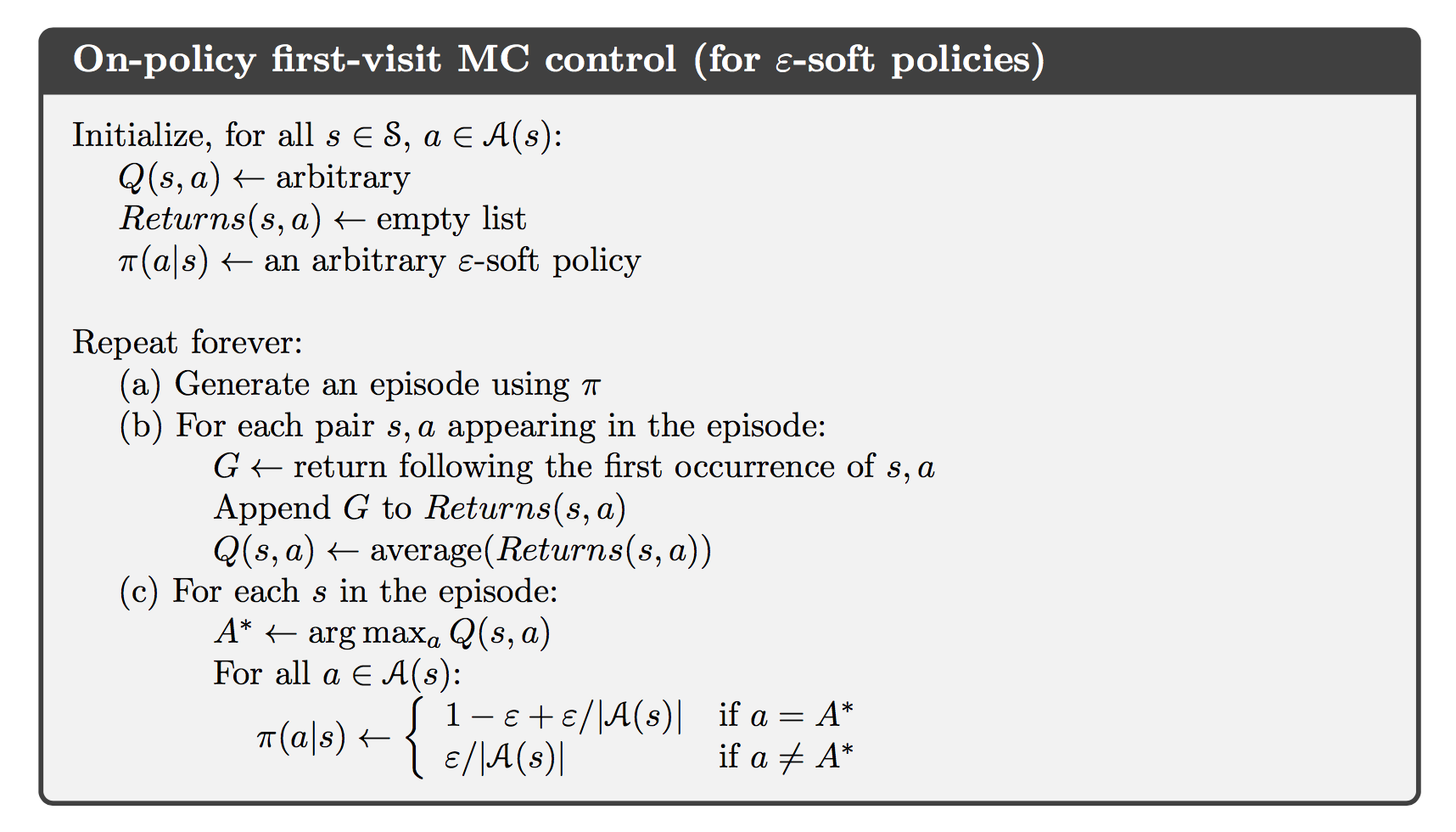
Monte Carlo Control without Exploring Starts

The only general way to ensure that all actions are selected infinitely often is for the agent to continue to select them. There are two approaches to ensuring this, resulting in what we call on-policy methods and off-policy methods. On-policy methods attempt to evaluate or improve the policy that is used to make decisions, whereas on-policy methods evaluate or improve a policy different from that used to generate the data.

In on-policy control methods the policy is generally soft, meaning that $\pi(a \vert s)>0$ for all $s\in\mathcal{S}$ and all $a\in\mathcal{A}(s)$, but gradually shifted closer and closer to a deterministic optimal policy.

Off-policy Prediction via Importance Sampling

All learning control methods face a dilemma: They seek to learn action values conditional on subsequent optimal behavior, but they need to behave non-optimally in order to explore all actions (to find the optimal actions). How can they learn about the optimal policy while behaving according to an exploratory policy? The on-policy approach in the preceding section is actually a compromise. It learns action values not for the optimal policy, but for a near-optimal policy that still explores. A more straightforward approach is to use two policies, one that is learned about and that becomes the optimal policy, and one that is more exploratory and is used to gen- erate behavior. The policy being learned about is called the target policy, and the policy used to generate behavior is called the behavior policy. In this case we say that learning is from data “off” the target policy, and the overall process is termed off-policy learning.

Suppose we wish to estimate $v_\pi$ or $q_\pi$, but we have all we have are episodes following another policy $\mu$, where $\mu \ne \pi$. In this case, $\pi$ is the target policy, $\mu$ is the behavior policy, and both policies are considered fixed and given. We require that $\pi(a \vert s)>0$ implies $\mu(a \vert s)>0$. This is called the assumption of coverage.

Almost all off-policy methods utilize importance sampling, a general technique for estimating expected values under one distribution given samples from another. Given a starting state $S_t$, the probability of the subsequent state-action trajectory, $A_t,S_{t+1},A_{t+1},\dots,S_T$, occurring under any policy $\pi$ is

$$\prod_{k=t}^{T-1}\pi(A_k|S_k)p(S_{k+1}|S_k,A_k).$$

Thus, the relatvie probability of the trajectory under the target and behavior policies (the importance-sampling ratio) is

$$\rho_t^T=\prod_{k=t}^{T-1}\frac{\pi(A_k|S_k)}{\mu(A_k|S_k)}.$$

We can define the set of all time steps in which state is visited, denoted $\mathcal{J}(s)$. This is for an every-visit method; for a first-visit method, $\mathcal{J}(s)$ would only include time steps that were first visits to $s$ within their episodes. Also, let $T(t)$ denote the first time of termination following time $t$, and $G_t$ denote the return after $t$ up through $T(t)$. Then $\{G_t\}_{t\in\mathcal{J}(s)}$ are the returns that pertain to state $s$, and $\{\rho_t^{T(t)}\}_{t\in\mathcal{J}(s)}$ are the corresponding importance-sampling ratios. To estimate $v_{\pi}(s)$, we simply scale the returns by the ratios and average the results:

$$V(s)=\frac{\sum _{t\in\mathcal{J}(s)}\rho_t^{T(t)}G_t}{\lvert\mathcal{J}(s)\rvert}.$$

When importance sampling is done as a simple average in this way it is called ordinary importance sampling.

An import alternative iis weighted importance sampling, which uses a weighted average, defined as

$$V(s)=\frac{\sum _{t\in\mathcal{J}(s)}\rho_t^{T(t)}G_t}{\sum_{t\in\mathcal{J}(s)}\rho_t^{T(t)}},$$

or zero if the denominator is zero.

The difference between the two kinds of importance sampling is expressed in their biases and variances. The ordinary importance-sampling estimator is unbiased whereas the weighted importance-sampling estimator is biased. On the other hand, the variance of the ordinary importance-sampling estimator is in general unbounded because the variance of the ratios can be unbounded, whereas in the weighted estimator the largest weight on any single return is one. In fact, assuming bounded returns, the variance of the weighted importance-sampling estimator converges to zero even if the variance of the ratios themselves is infinite. In practice, the weighted estimator usually has dramatically lower variance and is strongly preferred.

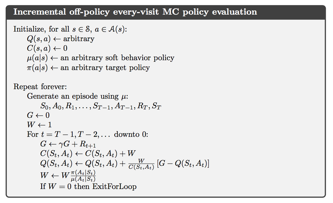
Incremental Implementation

Suppose we have a sequence of returns $G_1, G_2, \dots, G_{n-1}$, all starting in the same state and each with a corresponding random weight $W_i$ (e.g., $W_i=\rho_t^{T(t)}$).

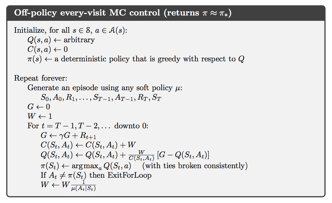
Off-Policy Monte Carlo Control