Temporal-difference (TD) learning is a combination of Monte Carlo ideas and dynamic programming (DP) ideas.

TD Prediction

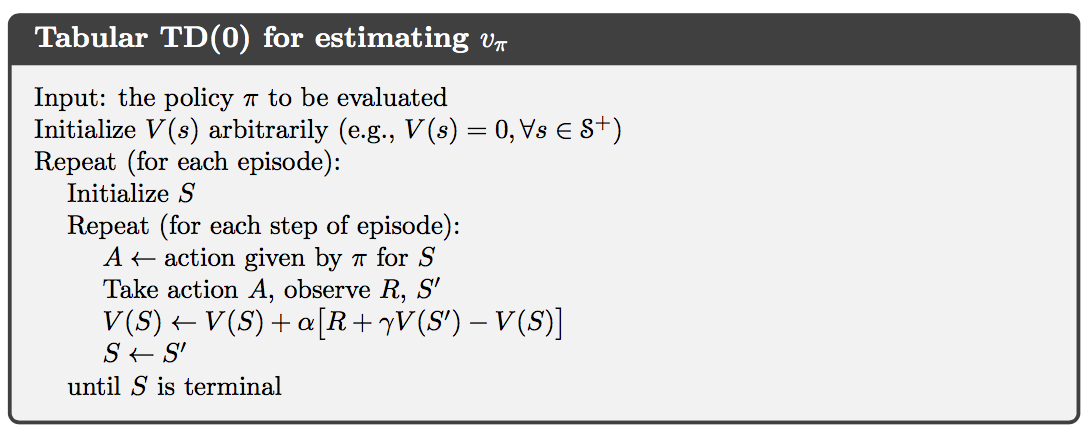
Both TD and Monte Carlo methods use experience to solve the prediction problem. Given some experience following a policy $\pi$, both methods update their estimate $v$ of $v_\pi$ for the nonterminal states $S_t$ occurring in that experience. Whereas Monte Carlo methods must wait until the end of the episode to determine the increment to $V(S_t)$ (only then is $G_t$ known), TD methods need wait only until the next time step. The simplest TD method, known as TD(0), is

$$V(S_t) = V(S_t) + \alpha[R_{t+1}+\gamma V(S_{t+1})-V(S_t)].$$

TD methods combine the sampling of Monte Carlo with the bootstrapping of DP. As we shall see, with care and imagination this can take us a long way toward obtaining the advantages of both Monte Carlo and DP methods.

Note that the quantity in brackets in the TD(0) update is a sort of error, measuring the difference between the estimated value of $S_t$ and the better estimate $R_t+\gamma V(S_{t+1})$. This quantity, called the TD error, arises in various forms throughout reinforcement learning:

$$\delta_t=R_{t+1}+\gamma V(S_{t+1})-V(S_t).$$

Also note that the Monte Carlo error can be written as a sum of TD errors:

$$\begin{split} G_t - V(s_t) &= R_{t+1}+\gamma G_{t+1} - V(S_t) + \gamma V(S_{t+1}) - \gamma V(S_{t+1}) \\ &= \delta_t + \gamma (G_{t+1}-V(S_{t+1})) \\ &= \delta_t + \gamma \delta_{t+1} + \dots + \gamma^{T-t} (G_T - V(S_T))\\ &= \sum_{k=0}^{T-t-1}\gamma^k\delta_{t+k} \end{split}$$

This fact and its generalizations play important roles in the theory of TD learning.

Optimality of TD(0)

Suppose there is available only a finite amount of experience, say 10 episodes or 100 time steps. In this case, a common approach with incremental learning methods is to present the experience repeatedly until the method converges upon an answer. Updates are made only after processing each complete batch of training data. We call this batch updating.

Batch Monte Carlo methods always find the estimates that minimize mean-squared error on the training set, whereas batch TD(0) always finds the estimates that would be exactly correct for the maximum-likelihood model of the Markov process. In this case, the maximum-likelihood estimate is the model of the Markov process formed in the obvious way from the observed episodes: the estimated transition probability from $i$ to $j$ is the fraction of observed transitions from $i$ that went to $j$, and the associated expected reward is the average of the rewards observed on those transitions. Given this model, we can compute the estimate of the value function that would be exactly correct if the model were exactly correct. This is called the certainty-equivalence estimate because it is equivalent to assuming that the estimate of the underlying process was known with certainty rather than being approximated. In general, batch TD(0) converges to the certainty-equivalence estimate.

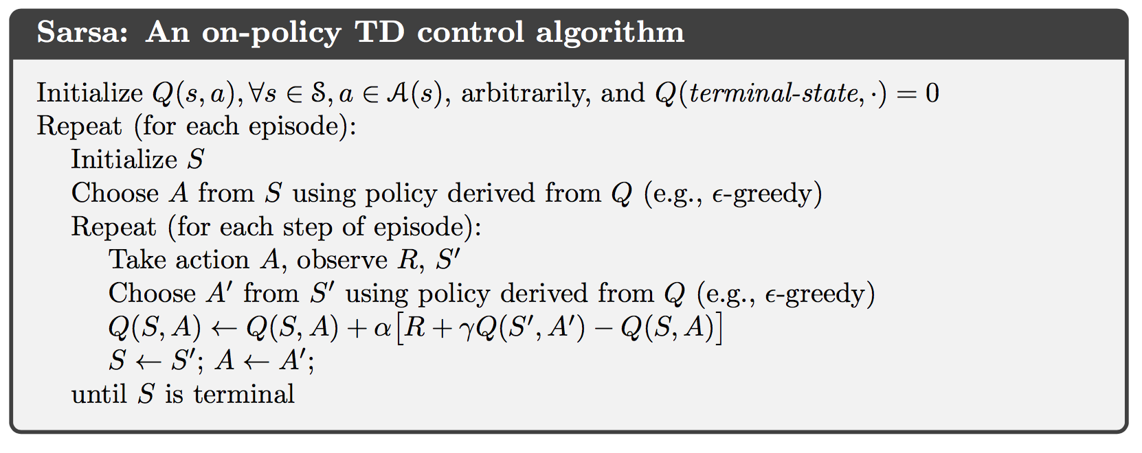
Sarsa: On-Policy TD Control

As usual, we follow the pattern of generalized policy iteration (GPI), only this time using TD methods for the evaluation or prediction part.

In the previous section we considered transitions from state to state and learned the values of states. Now we consider transitions from state–action pair to state–action pair, and learn the values of state–action pairs. The theorems assuring the convergence of state values under TD(0) also apply to the corresponding algorithm for action values:

$$Q(S_t,A_t)=Q(S_t,A_t)+\alpha[R_{t+1}+\gamma Q(S_{t+1},A_{t+1}) - Q(S_t, A_t)].$$

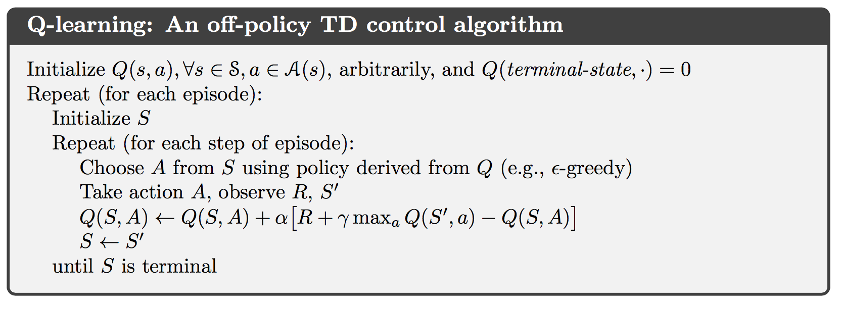
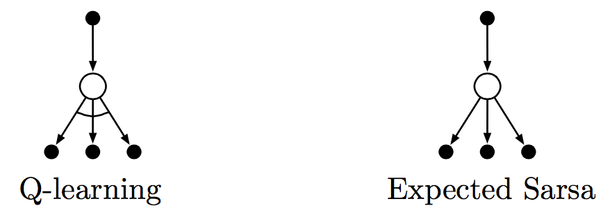
Q-learning: Off-Policy TD Control

One of the early breakthroughs in reinforcement learning was the development of an off-policy TD control algorithm known as Q-learning, defined by:

$$Q(S_t, A_t)=Q(S_t, A_t)+\alpha[R_{t+1}+\gamma\max_aQ(S_{t+1},a)-Q(S_t,A_t)]$$

In this case, the learned action-value function, $Q$, directly approximates $q^*$, the optimal action-value function, independent of the policy being followed.

Expected Sarsa

Consider the algorithm with the update rule:

$$\begin{split} Q(S_t,A_t)&=Q(S_t,A_t)+\alpha\left[R_{t+1}+\gamma \mathbb{E}[Q(S_{t+1},A_{t+1})|S_{t+1}]-Q(S_t,A_t)\right]\\ &=Q(S_t,A_t)+\alpha\left[R_{t+1}+\gamma\sum_a\pi(a|S_{t+1})Q(S_{t+1},a)-Q(S_t,A_t)\right] \end{split}$$

but that otherwise follows the schema of Q-learning. Given the next state $S_{t+1}$, this algorithm moves deterministically in the same direction as Sarsa moves in expectation, and accordingly it is called expected Sarsa.

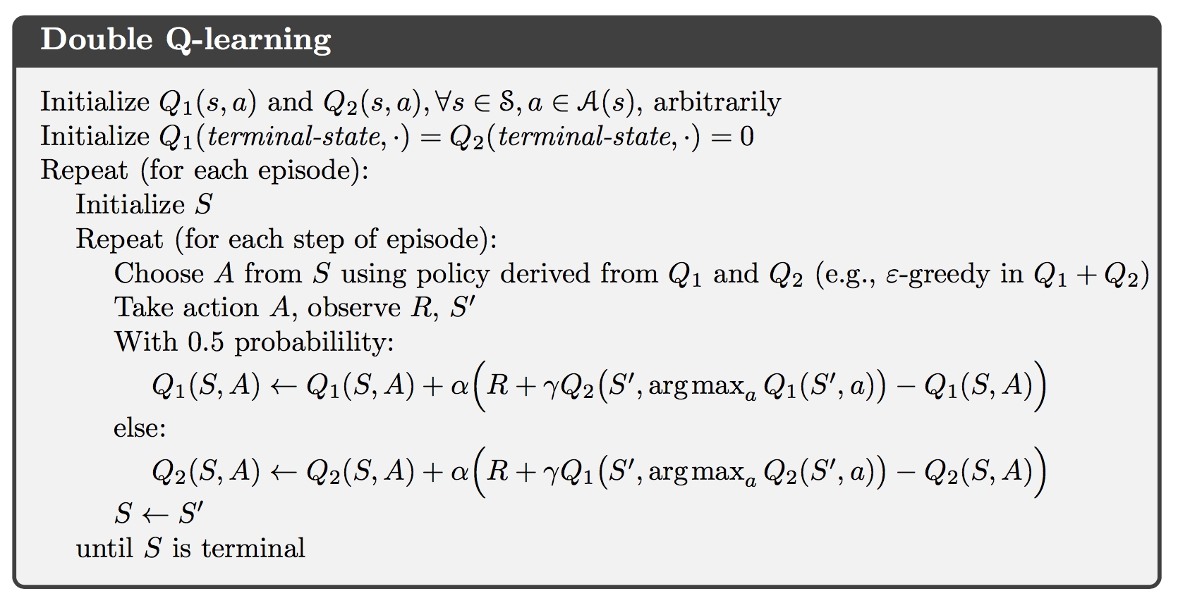
Maximization Bias and Double Learning

All the control algorithms that we have discussed so far involve maximization in the construction of their target policies. In these algorithms, a maximum over estimated values is used implicitly as an estimate of the maximum value, which can lead to a significant positive bias. We call this maximization bias.

One way to view the problem is that it is due to using the same samples (plays) both to determine the maximizing action and to estimate its value. Suppose we divided the plays in two sets and used them to learn two independent estimates, call them $Q_1(a)$ and $Q_2(a)$, each an estimate of the true value $q(a)$, for all $a\in\mathcal{A}$. We could then use one estimate, say $Q_1$, to determine the maximizing action $A^*=\mathrm{argmax}_aQ_1(a)$, and the other, $Q_2$, to provide the estimate of its value, $Q_2(A^*)=Q_2(\mathrm{argmax}_aQ_1(a))$. This estimate will then be unbiased in the sense that $\mathbb{E}[Q_2(A^*)]=q(A^*)$. We can also repeat the process with the role of the two estimates reversed to yield a second unbiased estimate $Q_1(A^*)=Q_1(\mathrm{argmax}_aQ_2(a))$. This is the idea of doubled learning.