Billy Ian's Short Leisure-time Wander

into learning, investment, intelligence and beyond

[Notes on Mathematics for ESL] Chapter 4: Linear Methods for Classification

| Comments

4.3 Linear Discriminant Analysis

Derivation of Equation (4.9)

For that each class’s density follows multivariate Gaussian

Take the logarithm of $f_k(x)$, we get

where $c = -\log [(2\pi)^{p/2}\lvert\Sigma\rvert^{1/2}]$ and $\mu_k^T\Sigma^{-1}x=x^T\Sigma^{-1}\mu_k$. Following the above formula, we can derive Equation (4.9) easily

[Notes on Mathematics for ESL] Chapter 3: Linear Regression Models and Least Squares

| Comments

3.2 Linear Regression Models and Least Squares

Derivation of Equation (3.8)

The least squares estimate of $\beta$ is given by the book’s Equation (3.6)

From the previous post, we know that $\mathrm{E}(\mathbf{y})=X\beta$. As a result, we obtain

Then, we get

The variance of $\hat \beta$ is computed as

If we assume that the entries of $\mathbf{y}$ are uncorrelated and all have the same variance of $\sigma^2$, then $\mathrm{Var}(\varepsilon)=\sigma^2I_N$ and the above equation becomes

This completes the derivation of Equation (3.8).

[Notes on Mathematics for ESL] Chapter 2: Overview of Supervised Learning

| Comments

2.4 Statistical Decision Theory

Derivation of Equation (2.16)

The expected predicted error (EPE) under the squared error loss:

Taking derivatives with respect to $\beta$:

In order to minimize the EFE, we make derivatives equal zero which gives Equation (2.16):

Note: $x^T\beta$ is a scalar, and $\beta$ is a constant.

统计释疑(3):大数定理和中心极限定理

| Comments

两个必须得记住并理解的统计学定理:大数定理和中心极限定理。有相当多的统计学理论是以这两个定理为基础。另外从我个人理解,这两个定理在一定程度上解释了为什么数据越多越好(为什么我们需要大数据)。

收敛的类型

为了更加准确的理解上述两个定理,我们需要理解概率层面的收敛,而非微积分里的收敛(如果对与任意$\epsilon>0$和足够大的$n$,$\vert x_n -x \rvert < \epsilon$,那么我们称这一实数列$x_n$收敛于极限$x$)。

在统计中,主要有两种类型的收敛:

统计释疑(2):概率不等式有什么用?

| Comments

在学习概率论或者一些统计课程的时候,往往会学到一系列各式各样稀奇古怪的不等式 (Inequalities),然而却对于这些不等式的意义缺乏一个直观的认识。引申“All of Statistics”一书中的一个小例子可以给出一个很切合实际的解释。

我的神经网络真的有效吗?

假如我们用神经网络在MNIST数据集上训练了一个分类器,我们在测试集上得到了一个错误率,比如$0.05$。那么这是否意味着我们可以保证我们的神经网络一定能达到$95\%$的正确率呢?显然训练一次得出的结果是不可靠的。那么,我们有多大的把握(概率)来相信这一观察到的错误率呢?

这时候就需要一些统计的语言了:假设我们有$n$个测试样本,每个测试样本分类的正确与否都是一个随机变量$X_1,\dots,X_n$。如果分类错误$X_i=1$,否则$X_i=0$。显而易见,$\bar X_n=n^{-1}\sum_{i=1}^nX_i$就是观察到的错误率。我们可以把每个$X_i$当做一个均值为$p$服从Bernoulli分布的随机变量,从而$p$就是真正(但是永远无法准确知晓)的错误率。从我们的角度来看,我们希望$\bar X_n$应该接近$p$。那么$\bar X_n$和$p$的概率超过一个固定值$\epsilon$的概率有多大呢? 这个概率就是$\mathbb{P}(\lvert\bar X_n -p\rvert > \epsilon)$,通常我们很难直接计算出它的值,这时我们就需要不等式来给这个概率设定一些边界 (bound)。

统计释疑(1):什么是p值

| Comments

某互联网公司招聘程序员,招聘的方法很简单,就是从LeetCode上找$10$道题,录取解出至少$8$道题的应试者。每隔一年,公司会根据新招聘程序员的表现评估上一年招聘的不合格率。公司的期望是每年招聘的不和格率要低于$5\%$。下面是历年的招聘数据:

年份 面试人数 录取人数 不合格的人数 不合格率
2014 1000 350 30 8.57%
2015 1000 650 10 1.54%
2016 1000 200 10 5.00%

那么这家公司的招聘策略是否有效呢?

【失控:机器、社会与经济的新生物学】漫谈(二)

| Comments

随着人工智能大潮的火热,各种噱头在大公司和媒体的鼓吹下刺激着大众的神经。关于智械的各种“浪漫”幻想也不再仅仅诉诸于电影和小说,而是开始被严肃的讨论了起来。在这本书里,我看到了一个之前没有见过的有趣的观点:“机器是人类的一种进化形式”。显然这并非通常的经过亿万年自然选择产生的进化,而是一种定向的选择。就如同培育有机食品、杂交水稻一般,人工智能是否也可以定向的让人类自身变得更为强大呢?相比于制造通用智能,越来越多业界的人也都认为AI被定义为Augmented Intelligence(增强智能)而非Artifical Intelligence(人工智能)更加实际和贴切。总的来说,现在的AI还是高度面向任务的,大量人工标注的数据加上工程上的细节才能使计算机在特定任务上战胜人类,而这些努力一旦换了一个领域就难再有大的用武之地。另一方面,希望计算机或者机器人在某些领域完全取代人类也是不现实的,除了一些很基础的任务外,人类的介入在现阶段还是很有必要的,比如机器翻译,智能助理等等。

【失控: 机器、社会与经济的新生物学】漫谈(一)

| Comments

重拾阅读后的第一本书,读而不思则罔,于是决定随着阅读随便写点什么,谓之“漫谈”。

虽然成书于94年,但书中种种观点和当今社会与技术的发展却有诸多不谋而合之处。读罢前几章,最为深刻的印象就是蜂群思维,分布式系统,去中心化等等一系列相关的概念。总而言之,论述的是一种与传统自上而下的系统相悖的自下而上的系统。这里的系统是一个非常宽泛的说法,它可以是机器,可以是软件,也可以是动物,乃至于人类社会、政治体系、万维网等等。可能是我实在是孤陋寡闻,在阅读这本书之前,我潜意识里确实认为绝大多数系统都应该有一个中心,拥有绝对的权威并下达指令,比如PC的CPU,古代的皇帝,人的大脑等等。然而这本书却提出了一个截然不同的系统,简而言之就是没有一个绝对的中心,每一个个体的行为决定了整体的行动(也可以简单的理解为少数服从多数,但实际情况往往更加复杂)并由简单的行为(操作)逐层向上模块化的增加更加复杂的行为(操作),另外分布式的存在方式令其拥有更强的容错性和在部分失灵的情况下能够继续运转的稳定性。现代科学在群体动物(蜂群、蚁群)中发现了这样的系统,而脑科学的发展也说明大脑并非我们原本想象的那样控制着人体的一切。无数的神经的共同作用造就了大脑,而大脑与身体的各种感官也似乎并非简单的从属关系。

Notes on Reinforcement Learning (4): Temporal-Difference Learning

| Comments

Temporal-difference (TD) learning is a combination of Monte Carlo ideas and dynamic programming (DP) ideas.

TD Prediction

Both TD and Monte Carlo methods use experience to solve the prediction problem. Given some experience following a policy $\pi$, both methods update their estimate $v$ of $v_\pi$ for the nonterminal states $S_t$ occurring in that experience. Whereas Monte Carlo methods must wait until the end of the episode to determine the increment to $V(S_t)$ (only then is $G_t$ known), TD methods need wait only until the next time step. The simplest TD method, known as TD(0), is

TD methods combine the sampling of Monte Carlo with the bootstrapping of DP. As we shall see, with care and imagination this can take us a long way toward obtaining the advantages of both Monte Carlo and DP methods.

Alt text

Notes on Reinforcement Learning (3): Monte Carlo Methods

| Comments

Monte Carlo methods are ways of solving the reinforcement learning problem based on averaging sample returns. To ensure that well-defined returns are available, here we define Monte Carlo methods only for episodic tasks.

Monte Carlo Prediction

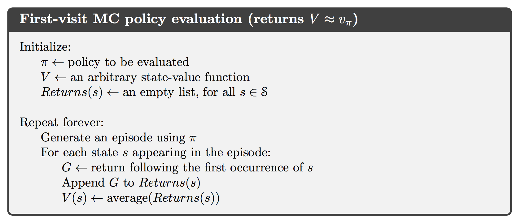
An obvious way to estimate the state-value function which is the expected return starting from that state from experience, is to average the returns observed after visits to that state. This idea underlies all Monte Carlo methods.

In particular, suppose we wish to estimate $v_\pi(s)$, the value of a state $s$ under policy $\pi$, given a set of episodes obtained by following $\pi$ and passing through $s$. Each occurrence of state $s$ in an episode is called a visit to $s$. The first-visit MC method estimates $v_\pi(s)$ as the average of the returns following from first visits to $s$, whereas every-visit MC method averages the returns following all visits to $s$.

Alt text