Billy Ian's Short Leisure-time Wander

into learning, investment, intelligence and beyond

Notes on Reinforcement Learning (2): Dynamic Programming

| Comments

Policy Evaluation

Consider a sequence of approximate value functions $v_0, v_1, v_2, \dots,$ each mapping $\mathcal{S}^+$ to $\mathbb{R}$. The initial approximation, $v_0$ is chosen arbitrarily, and each successive approximation is obtained by using the Bellman equation for $v_\pi$ as an update rule:

for all $s\in\mathcal{S}$.

Alt text

Notes on Reinforcement Learning (1): Finite Markov Decision Processes

| Comments

The Agent-Environment Interface

Alt text

  • The agent and environment interact at each of a sequence of discrete time steps, $t=0,1,2,3,\dots$
  • At each time step $t$, the agent receives some representation of the environment’s state, $S_t\in\mathcal{S}$, where $\mathcal{S}$ is the set of possible states.
  • On that basis, the agent selects an action, $A_t \in \mathcal{A}(S_t)$, where $\mathcal{A}(S_t)$ is the set of actions available in state $S_t$.
  • One time step later, in part as a consequence of its action, the agent receives a numerical reward, $R_{t+1} \in \mathcal{R} \subset \mathbb{R}$, and finds itself in a new state, $S_{t+1}$.

ML With R (3): Logistic Regression

| Comments

Code in R for Coursera-ML and CMPUT466/551 in University of Alberta

This post refers to programming exercise 2 in Coursera-ML. All the code can be found in this repo.

setwd("~/Coding/R/CMPUT466/mlclass-ex2")
library(ggplot2)
library(R.matlab)
library(devtools)
source_url("https://raw.githubusercontent.com/ggrothendieck/gsubfn/master/R/list.R")

Logistic Regression

Visualizing the data

Use a scatter plot to visualize the data.

data <- read.csv("ex2data1.txt", header=FALSE)
X <- as.matrix(data[,c("V1", "V2")])
y <- as.matrix(data$V3)
ggplot(data, aes(x=V1, y=V2, col=factor(V3))) + 
  geom_point(shape=I(3), size=I(3)) +
  labs(x="Exam1 score", y="Exam2 score") +
  scale_color_manual(name="", labels=c("Not admitted", "Admitted"), values = c("blue", "red"))

ML With R (2): Regularized Linear Regression

| Comments

Code in R for Coursera-ML and CMPUT466/551 in University of Alberta

This post refers to programming exercise 5 in Coursera-ML. All the code can be found in this repo.

setwd("~/Coding/R/CMPUT466/mlclass-ex5")
library(ggplot2)
library(R.matlab)
library(devtools)
source_url("https://raw.githubusercontent.com/ggrothendieck/gsubfn/master/R/list.R")

Regularized Linear Regression

Visualizing the dataset

Use a scatter plot to visualize the data.

data <- readMat("ex5data1.mat")
X <- data$X
y <- data$y
Xtest <- data$Xtest
ytest <- data$ytest
Xval <- data$Xval
yval <- data$yval
df <- data.frame(X=X, y=y)
ggplot(df, aes(X, y, col="Training data")) + geom_point(shape=I(4), size=I(3)) +
  labs(x="Change in water level (x)", y="Water flowing out of the damn (y)") +
  scale_color_manual(guide=FALSE, values=c("Red"))

ML With R (1): Linear Regression

| Comments

Code in R for Coursera-ML and CMPUT466/551 in University of Alberta

This post refers to programming exercise 1 in Coursera-ML. All the code can be found in this repo.

setwd("~/Coding/R/CMPUT466/mlclass-ex1")
library(ggplot2)
library(MASS)

Linear regression with one variable

Plotting the Data

Use a scatter plot to visualize the data.

data <- read.csv("ex1data1.txt", header=FALSE)
ggplot(data, aes(V1, V2, col="Training data")) + 
  geom_point(shape=I(4), size=I(3)) + 
  labs(x="Population of City in 10,000s", y="Profit in $10,000s") +
  scale_color_discrete(guide=FALSE)

阶段性回顾与展望

| Comments

不知不觉已经到加拿大九个月了,虽然一路上磕磕绊绊,但一切似乎都在我预想的轨道上发展,实在有些出乎意料。新的一个学期就要开始了,居然有点踌躇满志的意思呢。

生活

回顾:一开始真的不算顺利,先是遇到一个不怎么样的房东,lease没到就被要求搬走,押金也被扣了。初来乍到,只能认栽了,接下来又稀里糊涂的接了一个快到期的lease,结果住了3个月又得搬家。不到半年就搬了两次家也是醉了……还有吃饭,理发都是不小的问题。不过慢慢的自理能力也上来了,现在基本上生活上已经问题不大了,现在做饭虽然算不上多好吃,但基本饿不死了,周末还可以做个大盘鸡,炖个羊肉汤什么的,剩饭也可以炒个蛋炒饭,感觉还是挺滋润的。不过刚过来的时候碳酸饮料喝的有点多,导致现在牙齿有点敏感,可惜国外看牙太贵了,有机会回国的话一定得把牙齿好好检查一下。

展望:碳酸饮料需要戒掉,甜食也尽量少吃;多多学习烹饪,尽量少出去吃些快餐;多注意一下形象管理,别太邋遢了;还有就是平时多注意锻炼,吃完饭犯困了,可以出去走走,玩会儿pokemon go~

Probabilistic Graphical Models (1): Introduction

| Comments

What is probabilistic graphical model (PGM)? Forget about some high-level and complicated sentences on textbook or wikipedia. From my perspective, it’s all about graphs, distributions and the connections between them.

There are three aspects to a graphical model:

  • The graph
  • A model of the data based on the graph
  • The data itself

Actually, the data is generated by the underlying distribution and the model is the connection between the graph and the distribution. Here comes three fundamental issues:

  • Representation: How to represent the three aspects mentioned above succinctly?
  • Inference: How do I answser questions/queries according to my model and the given data? For example, the probability of a certain variable given some observations $P(X_i \vert \mathcal{D})$.
  • Learning: What model is “right” for my data? We may want to “learn” the parameters of the model, or the model itself or even the topology of the graph from the data.

GSoC 2016: Inferring Infobox Template Class Mappings From Wikipedia and WikiData

| Comments

This page is the public project page and will be updated every week.

Project Description

There are many infoboxes on wikipedia. Here is a example about football box:

Alt text

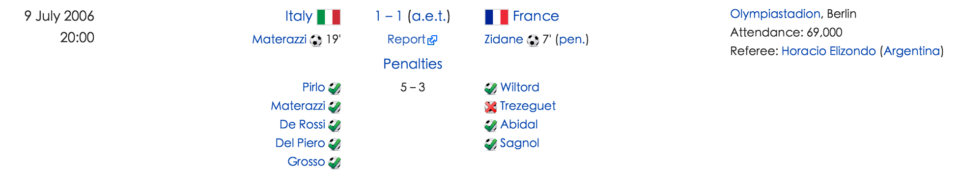
As seen, every infobox has some properties. Actually, every infobox follows a certain template. In my project, the goal is to find mappings between the classes (eg. dbo:Person, dbo:City) in the DBpedia ontology and infobox templates on pages of Wikipedia resources using techniques of machine learning.

There are lots of infobox mappings available for a few languages, but not as many for other languages. In order to infer mappings for all the languages, cross-lingual knowledge validation should also be considered.

The main output of the project will be a list of new high-quality infobox-class mappings.

Trace of My Study on Machine Learning

| Comments

This blog will record the timeline, resources, projects along the way of my study on machine learning since 2015. And I will keep updating this blog.

Mathematics

Machine Learning Basics(1): Linear Regression

| Comments

As a beginner in machine learning, I plan to sketch out my learning process. And it will be my first post in this series.

1. Definition

We have an input vector $X^T=(X_1, X_2, \dots, X_p)$ and want to predict a real-valued output $Y$. The linear regression model has the form

Here the $\beta_j$’s are unknown parameters or coefficients.